Bitboards
In order to write an efficient AI for Hidamari, my implementation of Tetris, first a representation of the game state that used very little memory had to be devised. Minimizing the size of the game state is crucial for state-space searches. A naive representation of a Tetris game state would be a 12x22 grid of bytes, each byte representing a different color block. While this isn’t excessive, only requiring 264 bytes total, it can be done better. Since colors of the blocks don’t matter for gameplay, really only one bit is needed to represent if a block is filled in the space on a board or not, not an entire byte. A bitboard, commonly found in Chess programs, can be used to save space here.
Normally used in chess programs to represent the board, a bitboard is a representation of the game state where each integer represents one row of the playfield, and the bits of each integer are the cells of that row. For example an 8x8 grid can be represented by 8 8-bit integers in an array.
An 8x8 bitboard
0 0 0 0 0 0 0 0
0 0 0 0 0 0 0 0
0 0 0 0 0 0 0 0
0 0 0 0 0 0 0 0
0 0 0 0 0 0 0 0
0 0 0 0 0 0 0 0
0 0 0 0 0 0 0 0
0 0 0 0 0 0 0 0
Since Hidamari uses a 12x22 grid, 16 bit integers must be used since most machines don’t have a 12 bit integer size. This reduces the space from the basic representation from 264 bytes to 44 bytes. This size reduction is beneficial for state-space searches that will be performed by the AI. Another benefit to switching to a bitboard representation is the simplification of the operations needed to be performed on the board to detect collision and perform piece movement. Collisions can be detected by AND-ing pieces with the board, and movement by OR-ing, both of which are fast bit-wise instructions.
One downside to representing the game state this way is that it necessitates additional layers of information to store colors and textures of the tiles on the playfield. This isn’t really a problem as it would be best to detach this information anyway, since the AI doesn’t need to concern itself over the color of the pieces. All it needs is the useful gameplay information to decide which moves to make.
Grid Structures in C
/* The old simple grid, 264 bytes */
uint8_t simple_grid[12][22];

/* The new bitboard representation, 44 bytes */
uint16_t bitboard[22];
Strategy
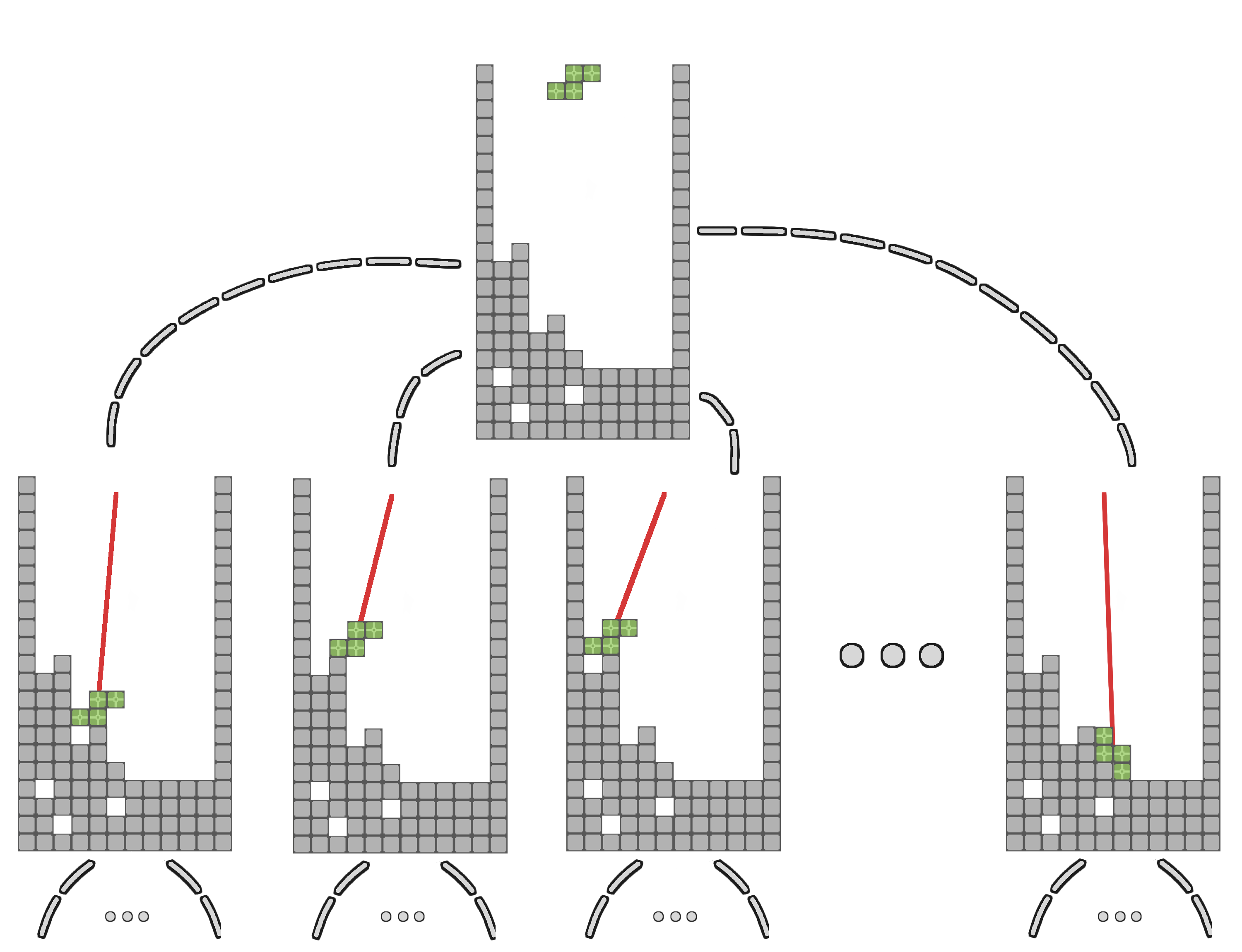
This section describes the state-space search strategy the AI in the above video uses, and the heuristic functions for choosing the best moves. The state-space search itself is a simple depth-first search through a fixed number of important states of the game. An important state is defined as the final locked in position of a piece, as illustrated:
Visualization of state space search
The depth-first search, as programmed, is computed every time a new piece is revealed at a depth of two, which means the positions for the current falling piece and the next piece are computed. This means the AI utilizes the knowledge of the next piece to determine where to place the currently falling piece, but does not lock itself into where it decides to place the next until its own next piece is previewed.
This depth-first search is very memory efficient using a static amount 180kb of memory for the entire search. A stack-allocation scheme is used for this fixed-size 180kb block of memory which allows for very quick allocation of states during the search, as fast as moving the stack pointer.
The method the AI uses to evaluate each important state is by running a set of heuristic scoring functions on the state and returning a score for the state derived from the scoring functions. Similar to golf, the higher the score, the less desirable the state. One the state with the lowest score has been found, the AI traces back up the state-space tree generated from the search to compute the plan to achieve that low-score state from the current state.
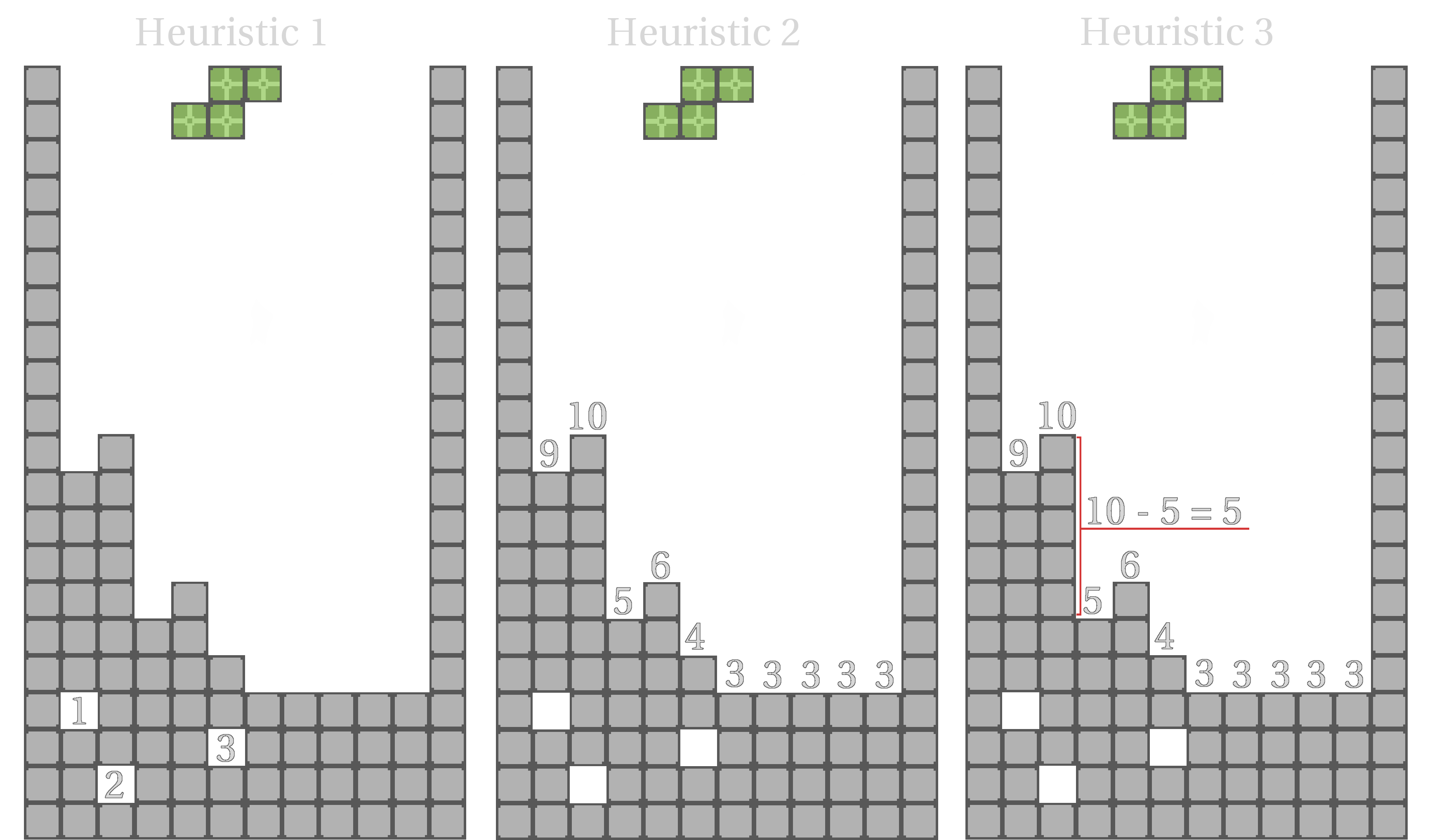
The first heuristic used is to count the number of “holes” in the playfield. A hole is defined as any open tile that has a tile above it anywhere in the same column. Each hole is difficult to fill, since it would require clearing all the lines above it, they should be avoided whenever possible.
The second heuristic used sums the height of each column. Keeping the aggregate height of the field is desirable, as once the 20 height limit is broken the game ends.
The third heuristic used sums the difference in height of each column and its neighbor. This creates a “bumpiness” value. A bumpy playfield is undesirable, as it makes fitting most pieces more difficult.
Each of the heuristics is given a weighting deemed on its importance. For instance, the “holes” heuristic gets a multiplier of 10 times, since holes are very undesirable, and the other two attributes are less dangerous than holes. These multipliers can be adjusted to make the AI perform better or worse. The current multipliers were discovered through a small amount of trial and error, however another program could be written to optimize these values for us.
Optimization
In order to find optimal heuristic weights for the AI’s static evaluation function, particle swarm optimization was used. The particle swarm algorithm used is about the same as the one that can viewed on wikipedia. The gist of it is that a k particles are created to explore an n dimensional space, where n is the number of features in a function being optimized. In this case, with three heuristic weights as features, n is equal to 3. Each of the k particles simulates games of Tetris as a fitness function. Whichever ones play for the longest, scoring the highest fitness score, influence the rest of the swarm to move towards their coordinates and explore closer to their position in the search space.
Particle Swarm Optimization is usually a serial algorithm, which means computing the score for each particles’ positions, and then moving them all in order. This would take forever to complete a single iteration if the scoring function being used was a game of Tetris, as each particle would have to wait for the previous one to finish playing before it could start playing Tetris. Rather than doing this serially, I modified the algorithm to be asynchronous by allowing t particles to be playing Tetris on separate threads at the same time, where t is the number of threads specified. In addition, particles were queued up in a thread-safe priority queue where the particles with the least amount of iterations were at the head of the queue. This ensured that the particles would be processed in a somewhat balanced manner and ensure that some particles didn’t complete all of their iterations far before the rest.
Video demonstration of Particle Swarm
A fitness of over 500,000 lines cleared could be considered as playing indefinitely, since this amounts to a score of around 500,000,000 points in most Tetris games, where getting 1,000,000 points is considered impressive amongst even very skilled players. The swarm ended up finding multiple weights that allowed the AI to play for 500,000 lines and gain 500,000,000 points. The weights found using particle swarm optimization to achieve this score are:
| Heuristic | Description | Weight |
|---|---|---|
| 0 | total column height | 0.848058 |
| 1 | total column difference | 2.304684 |
| 3 | total number of holes | 1.405450 |
These weights were computed with a 200 particle swarm with each particle performing 100 iterations. Even with 4 CPUs used to parallelize the computation it took days to complete. This was due to the fact that higher fitness scores simply required longer to compute, since a high fitness meant playing Tetris for a longer period of time. Although the particle swarm was able to find fairly good weights early on into the computation, so much of the duration of the process was simply refining the particles to converge.
Final Paper
This post was made using work I did for my AI class at UNH. The paper can be downloaded and read here. Hope you enjoy reading it!